
Optimization and Complexity: The Cost of Complexity [Systems thinking & modelling series]
This is part 63 of a series of articles featuring the book Beyond Connecting the Dots, Modeling for Meaningful Results.
After a good deal of work and many sleepless nights you have completed the first draft of your Aquatic Hamster population model. The results are looking great and your friend is really impressed. When he runs it by some colleagues however, they point out that your model does not account for the effects of the annual Pink Spotted Blue Jay migration.
Pink Spotted Blue Jays (PSBJ) migrate every fall from northern Canada to Florida. In the spring they return from Florida to Canada. Along the way, they usually spend a few days by the lake where the Aquatic Hamsters have their last colony. During this time they eat the same Orange Hippo Toads the hamsters themselves depend on. By reducing the Hippo Toad population, the PSBJ negatively affect the hamsters, at least for this period of time when there is less food available to support them.
The timing of the PSBJ migration can vary by several weeks each year; no one knows precisely when the PSBJ’s will arrive at the lake or even how long they will stay there. Further, the population of migrating birds can fluctuate significantly with maybe 100 birds arriving one year and 10,000 another year. The amount of toads they eat is proportional to the number of birds. Not much data exist quantifying the birds’ effects on the hamsters, but it is a well-established fact that they eat the Hippo Toads the hamsters rely upon for their survival and many conservationists are concerned about the migration.
Your friend’s colleagues wonder why you have decided to not include the PSBJ migration in your model. They want to know how they can trust a model that does not include this factor that clearly has an effect on the hamster population.
In response, you may point out that though the migration clearly has an impact, it appears to be a small one that is not as important as the other factors in the model. You add that there are no scientific studies or theoretical basis to define exactly how the migration functions or how it affects the hamster population. Given this, you think it is probably best to leave it out.
You say all this, but they remain unconvinced. “If there is a known process that affects the hamster population, it should be included in the model,” they persist. “How can you tell us we shouldn’t use what we know to be true in the model? We know the migration matters, and so it needs to be in there.”
The Argument for Complexity
Your friend’s colleagues have a point. If you intentionally leave out known true mechanisms from the model, how can you ask others to have confidence in the model? Put another way, by leaving out these mechanisms you ensure the model is wrong. Wouldn’t the model have to be better if you included them?
On the surface this argument is quite persuasive. It innately makes sense and appeals to our basic understanding of the world: Really it seems to be “common sense”.
It is also an argument that is wrong and very dangerous.
Before we take apart this common sense argument piece by piece, let us talk about when complexity is a good thing. As we will show, complexity is not good from a modeling standpoint, but it can sometimes be a very good tool to help build confidence in your model and to gain support for the model.
Take the case of the PSBJ migration. It might be that adding a migration component to the model ends up not improving the predictive accuracy of the model. However, if other people view this migration as important, you may want to include the migration in the model if for no other reason than to get them on board. Yes, from a purely “prediction” standpoint it might be a waste of time and resources to augment the model with this component, but this is sometimes the cost of gaining support for a model. A “big tent” type model that brings lots of people on board might not be as objectively good as a tightly focused model, but if it can gain more support and adoption it might be able to effect greater positive change.
The Argument Against Complexity
Generally speaking, the costs of complexity to modeling are threefold. Two are self evident: there are computational costs to complex models, as they take longer to simulate, and there are cognitive costs, in that they are harder to understand. There is, however, a third cost to complexity that most people do not initially consider: complex models are often less accurate than simpler ones.
In the following sections we detail each of these three costs.
Computational Performance Costs
As a model becomes more complex, it takes longer to simulate. When you start building a model it may take less than a second to complete a simulation. As the model’s complexity grows, the time required to complete a simulation may grow to a few seconds, then to a few minutes, and possibly even a few hours or more.
Lengthy simulation times can significantly impede model construction and validation. The agile approach to model development we recommend is predicated on rapid iteration and experimentation. As your simulation times cross beyond even something as small as 30 seconds, model results will no longer be effectively immediate and your ability to rapidly iterate and experiment will be diminished.
Furthermore, when working with an optimizer or sensitivity-testing tool, performance impacts can have an even larger effect. An optimization or sensitivity testing tool may run the model thousands of times or more in its analysis, so even a small increase in the computation time for a single simulation may have a dramatic impact when using these tools.
Optimizations themselves are not only affected by the length of a simulation, they are also highly sensitive to the number of parameters being optimized. You should be extremely careful about increasing model complexity if this requires the optimizer to adjust additional parameter values. A simplistic, but useful, rule of thumb is that optimization time increases tenfold for every parameter to be optimized.1
Thus, if it takes one minute to find the optimal value for one parameter, it takes 10 minutes to find the optimal values for two parameters and 100 minutes to find the optimal values for three parameters. Imagine we had built a model and optimized five parameters at once. We have increased the model complexity so we now have to optimize ten parameters. Our intuition would be that the optimization would now take twice as long. This is wrong. Using our power of ten rule we know that the time needed will be closer to 10^5 or 100,000 times as long!
That is a huge difference and highlights the importance of managing model complexity. A rule of thumb is that you should have no difficulty optimizing one or two parameters at a time. As you add more parameters, the optimization task becomes rapidly more difficult. At approximately five parameters you have a very difficult but generally tractable optimization challenge. Above five parameters you may be lucky to obtain good results.
Cognitive Costs
In addition to the computational cost of complexity, there is also a cognitive cost. As humans we have a finite ability to understand systems and complexity. This is partly why we model in the first place: to help us simplify and understand a world that is beyond our cognitive capacity.
Let’s return to our hamster population model. Including the bird migration could make it more difficult to interpret the effects of the components of the model and extract insights from them. If we observe an interesting behavior in the expanded model we will have to do extra work to determine if it is due to the migration or some other part of the model. Furthermore, the migration may obscure interesting dynamics in the model, making it more difficult for us to understand the key dynamics in the hamster system and develop insights from the model.
We can describe this phenomenon using a simple conceptual model defined by three equations. The number of available insights in a model is directly proportional to model complexity. As the model complexity increases, the number of insights available in the model also grows.
![]()
Conversely, our ability to understand the model and extract insights from it is inversely proportional to model complexity. α is a constant indicating the degree to which understandability decreases as complexity increases. This relationship is non-linear, as each item added to a model can interact with every other item currently in the model. Thus, the cognitive burden increases exponentially as complexity increases.
![]()
The number of insights we actually gain from a model is the product of the number of available insights and our ability to understand the model:
![]()
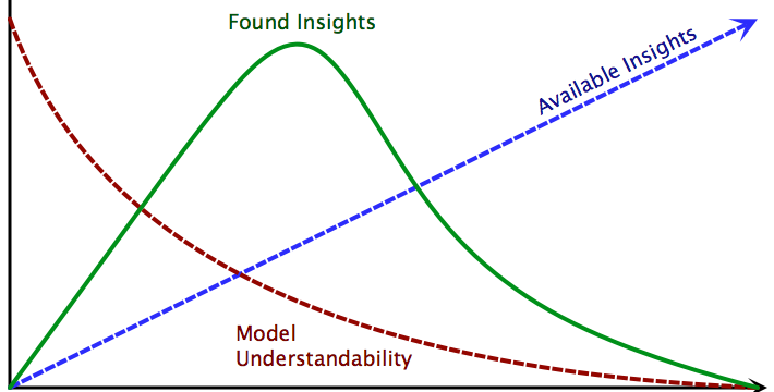
Thus when the model complexity is 0 – in effect basically no model – we gain no insights from the model. As the model complexity increases we begin to gain additional insights. After a certain point however, the added model complexity actually inhibits additional understanding. As complexity rises our insights will fall back down towards 0. This phenomenon is illustrated in Figure 1.
Accuracy Costs
The negative effects of complexity on computational performance and our cognitive capacity should not be a surprise. On the other hand, what may be surprising is the fact that complex models are in fact often less accurate than simpler alternatives.
To illustrate this phenomenon, let us imagine that for part of our hamster population model we wanted to predict the size of the hamsters after a year.2 The hamsters go through two distinct life stages in their first year: an infant life stage that lasts 3 months and a juvenile life stage that lasts 9 months. The hamsters’ growth patterns are different during each of these periods.
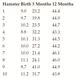
Say a scientific study was conducted measuring the sizes of 10 hamsters at birth, at 3 months, and at 12 months. The measurements at birth and at 12 months are known to be very accurate (with just a small amount of error due to the highly accurate scale used to weigh the hamsters). Unfortunately, the accurate scale was broken when the hamsters were weighed at 3 months and a less accurate scale was used instead for that period. The data we obtain from this study are tabulated below and plotted in Figure 2:
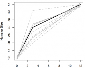
Now, unbeknownst to us, there is a pair of very simple equations that govern Aquatic Hamster growth. During the infant stage (first 3 months) they gain 200% of their birth weight. Their growth rate slows down once they reach the juvenile stage such that at the end of the juvenile stage their weight is 50% greater than it was when they completed the infant stage. Figure 2 plots this true (albeit unknown) size trajectory compared to the measured values. The higher inaccuracy of the measurements at 3 months compared to 0 and 12 months is readily visible in this figure by the greater spread of measurements around the 3 month period.
We can summarize this relationship mathematically:
![]()
![]()
Naturally, we can combine these equations to directly calculate the weight of the hamsters at 12 months from their weight at birth:
![]()
Again, we don’t know this is the relationship, so we need to estimate it from the data. All we care about is the size of hamsters at 12 months given their birth size. The simplest way to estimate this relationship is to do a linear regression estimating the final size as a function of the initial size. This regression would result in the following relationship:
![]()
This result is quite good. The estimated linear coefficient of 4.65 is very close to the true value of 4.50. So far our model is doing pretty well.
However, like with the bird migration, someone might point out that this model is too crude. “We know that the hamsters go through an infant and juvenile stage”, they might say, “we should model these stages separately so the model is more accurate.”
This viewpoint has actually been upheld in legal cases. For instance, there have been judicial decisions that “life-cycle” models, those that model each stage of an animal’s life are the only valid ones.3 If we were presenting this model to an audience that believed that, we would have to create two regressions: one for the infant stage and one for the juvenile stage.
Using the data we have, we would obtain these two regressions:
![]()
![]()
Combining these regression to get the overall size change for the 12 months we obtain the following:
![]()
Now, in this example we are fortunate to know that the true growth multiplier should be 4.50, so we can test the accuracy of our regressions. The error for this relatively detailed life-cycle model is (4.50-4.22)/4.50 or 6.2%. For the “cruder” model where we did not model the individual stages, the overall error is (4.50-4.65)/4.50 or 3.3%.
So by trying to be more accurate and detailed, we built a more complex model that has almost twice the error of our simpler model! Let’s repeat that: The more complex model is significantly less accurate than the simpler model.
Why is that? We can trace the key issue back to the problem that our data for the 3 month period are significantly worse than our data for 0 months or 12 months. By introducing this data into the model, we reduce the overall quality of the model by injecting more error into it. When someone asks you to add a feature to a model you have to consider if this feature may actually introduce more error into the model as it did in this example.
We can think of life-cycle and many other kinds of models as a chain. Each link of the chain is a sub-model that transforms data from the previous link and inserts them into the next. Like a chain, models may only be as good as their weakest link. It is often better to build a small model where all the links are strong, than a more complex model with many weak links.
| Exercise 9-9 |
|---|
| Implement a model tracking the growth of a hamster from birth to 12 months. Create the model for a single hamster and then using sensitivity testing to obtain a distribution of hamster size. Assume hamster are born with an average size of 10 and a standard deviation of 1. Use the true parameter growth rates and do not incorporate measurement uncertainty in the model. |
| Exercise 9-10 |
|---|
| Define a procedure for fitting a System Dynamics model of hamster growth to the hamster growth data in the table. Assume you know that there are two linear growth rates for the infant and juvenile stages but you do not know the values of these rates. |
| Exercise 9-11 |
|---|
| Apply the optimization procedure to your System Dynamics model to determine the hamster rates of growth from the empirical data. |
Overfitting
The act of building models that are too complex for the data you have is known as “overfitting” the data.4 In the model of hamster sizes, the model where we look at each life stage separately is an overfit model; we do not have the data to justify this complex of a model. The simpler model (ignoring the different stages) is superior.
Overfitting is unfortunately too common in model construction. This is partially because the techniques people use to assess the accuracy of a model are often incorrect and inherently biased to cause overfitting. To see this, let’s explore a simple example. Say we want to create a model to predict the heights of students in high school (this is seemingly trivial, but bear with us). To build the model we have data from five hundred students at one high school – “Mom’s High School” (Mom High).
We begin by averaging the heights of all the students at Mom High in our data set and find that the average student height is 5 feet 7 inches. That number by itself is a valid model for student height. It is a very simple model5, but it is a model nonetheless: Simply predict 5 feet 7 inches for the height of any student.
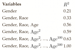
We know we can make this model more accurate. To start, we decide to create a regression for height, where gender is a variable. This gives us a new model that predicts women high-school students have a height of 5 feet 5 inches on average, while men have a height of 5 feet 9 inches on average. We calculated the R2 for the model to be 0.21.
That’s not bad, but for prediction purposes we can do better. We decide to include students’ race as a predictor, as we think that on average there might be differences in heights for different ethnicities. We complete this extended model including ethnic status as a predictor alongside gender and the R2 fit of our model increases to 0.33.
We think we can do even better, so we add age as a third predictor. We hypothesize that the older the students are, the taller they will be. The model including age as an additional linear variable is significantly improved with an R2 of 0.56.
Once we have built this model, we realize that maybe we should not just have a linear relationship with age because as students grow older, their rate of growth will probably slow down. To account for this we decide to also include the square of age in our regression. With this added variable our fit improves to an R2 of 0.59.
This is going pretty well; we might be on to something. But why stop with the square? What happens if we add higher order polynomial terms based on age? Why not go further and use the cube of age? The fit improves slightly again. We think we are on a roll and so we keep going. We add age taken to the fourth power, and then to the fifth power, and then to the sixth, and so on.
We get a little carried away and end up including 100 different powers of age. Each time we add a new power our R2 gets slightly better. We could keep going, but it’s time to do a reality check.
Do really we think that including AGE100 made our model any better than when we only had 99 terms based on age? According to the R2 metric it did (if only by a very small amount). However, intuitively we know it did not. Maybe the first few age variables helped, but once we get past a quadratic (AGE + AGE2) or cubic (AGE + AGE2 + AGE3) relationship, we probably are not capturing any more real characteristics of how age affects a person’s size.
So why does our reported model accuracy – R2 – keep getting better and better as we add these higher order power terms based on age to our regression?
This question is at the heart of overfitting. Let’s imagine taking our exploitation of age to its logical conclusion. We could build a model with 500 different terms based on age (AGE + AGE2 + AGE3 + … + AGE500). The result of this regression would go through every single point in our population of five hundred students.6 This model would have a perfect R2 of one (as it matches each point perfectly) but intuitively we know that it would be a horrible model.
Why is this model so bad? Imagine two students born a day apart. Today one has a height of 6 feet 2 inches the other has a height of 5 feet 5 inches. Our model would indicate that a single day caused a 9-inch difference in height. Even more ridiculous, the model would predict a roller coaster ride for students as they aged. According to the model they would gain inches one day and lose them the next. Clearly this model is nonsensical. However, this nonsensical model has a perfect R2. It is a paradox!
The key to unlocking the solution to the paradox and overcoming overfitting turns out to be surprisingly simple: assess the accuracy of a model using data that were not used to build the model.
The reason our overfit model for students looks so good using the R2 error metric is that we measured the R2 using the same data that we just used to build the model. Clearly this is an issue, as we can force an arbitrarily high R2 simply by continually increasing the complexity of our model. In this context the R2 we are calculating turns out to be meaningless.
What we need to do is to find new data – new students – to test our model on. That will be a more reliable test of its accuracy. If we first built our model, applied it to a different high school, and calculated the R2 using this new data, we would obtain a truer measure of how good our model actually was.
Figure 3 illustrates the effect of overfitting using observation from 9 students. The top three graphs plot the heights and ages for these nine students. We fit three models to these data: a simple linear one, a quadratic polynomial, and an equation with nine terms so that it goes through each point exactly.
Below the three graphs we show the regular R2 that most people use when fitting models, and what the true R27 would be if we applied the resulting model to new data. The regular R2 always increases, so if we used this naive metric we would always choose the most complex model. As we can see, the true accuracy of the model decreases after we reach a certain complexity. Therefore, in this case the middle model is really the better model. When illustrated like this, this concept of overfitting should make a lot of sense; but, surprisingly, it is often overlooked in practice even by modeling experts.

In general, overfitting should be watched for carefully. If you do not have a good metric of model error, the inclination to add complexity to your model will be validated by misleadingly optimistic measures of error that make you think your model is getting better, when it is actually getting worse. The optimization techniques we described earlier in this chapter are also susceptible to these problems, as every time you add a new variable to be optimized the optimization error will always decrease. The more parameters you add the worse this effect will be.
How do we estimate the true error of the model fit? The simplest approach is to split your dataset into two parts. Build the model with one half of the data and then measure the accuracy using the other half. With our high-school students we would randomly assign each dataset to be used either to build the model or to assess the model’s error. Advanced statistical techniques such as cross-validation or bootstrapping are other approaches and can be more effective given a finite amount of data. Unfortunately, we do not have space to discuss them here, but we would recommend exploring these on your own if you are interested in this topic.
No one ever got fired for saying, “Let’s make this model more complex.” After this chapter, we hope you understand why this advice, though safe to say, is often exactly the wrong advice.
| Exercise 9-12 |
|---|
| What is overfitting? What is underfitting? |
| Exercise 9-13 |
|---|
| You have been asked to evaluate a model built by a consulting company. The company tells you that their model has an R2 of 0.96 and is therefore a very accurate model.
Do you agree? What questions or tests do you need to do to determine if the model is good? |
Next edition: Modeling With Agents: Introduction.
Article sources: Beyond Connecting the Dots, Insight Maker. Reproduced by permission.
Notes:
- In practice an optimizer should ideally perform a bit better than this, but this provides a useful guideline to understand optimizations. Also, it should be noted that the optimizations we are talking about here are for non-linear optimization problems, for which gradients (derivatives) cannot be directly calculated. For other types of optimization problems, such as linear problems, much faster optimization techniques are available. ↩
- Size could affect hamster survival and fertility, so it could be an important variable to model. ↩
- Technically the determination is that life-cycle models are the “best available science”. These decisions are misguided and frankly wrong, but that is what occurs when judges are put in the position of making highly technical scientific decisions. ↩
- The reverse – building models that are too simple – is called “underfitting”. In practice, underfitting will be less of a problem, as our natural tendency is to overfit. ↩
- Statisticians would call this the “null” model, the simplest model possible. ↩
- Remember a polynomial equation with two terms can perfectly pass through two data points, an equation with three terms can perfectly pass through three points, and so on. ↩
- You might have heard of R2 variants such as the Adjusted R2. The Adjusted R2 is better than the regular R2; however it is important to note that it is not the true R2. Adjusted R2 also has some issues with overfitting. ↩

